Forget OLS Regression! Discover ExpectileGAM for Smarter Price Optimization (Part Two)

Unlocking the Potential of Computing the Price Elasticity of Demand, the Fun Way

Table of Content:

1. Recap of Part One

2. ExpectileGAM Model in Python

3. Price Optimization

4. Conclusion

Recap of Part One

In Part One, we learned that using OLS regression for price optimization is like going on just one coffee date and assuming you know everything about the person. But data is more mysterious than that! In Part Two, we’ll get up close and personal with ExpectileGAM, our ‘lady in veils,’ who helps us understand both the highs and lows of demand behavior for better price strategies. Ready to lift the veil?

ExpectileGAM Model in Python

I remember when I first encountered ‘ExpectileGAM’ — I thought, ‘What on earth is this?’ My brain was yelling, ‘Run!’ But instead, I decided to take a deep breath, embrace the discomfort, and dive in. Think of OLS as seeing only one side of a person, like a single date. ExpectileGAM, on the other hand, is like dating someone multiple times, with each ‘veil’ they lift revealing a different side of their personality — fun, serious, quiet, or quirky. ExpectileGAM lifts these ‘veils’ to capture the whole story of our data.

Here’s how it works in simpler steps:

ExpectileGAM uses expectiles to capture different levels in the data:

• The middle line represents the average pattern.

• The higher lines show how things behave when values are at their highest.

• The lower lines show what happens at the lowest values.

So, if we’re looking at prices and sales, the top expectile line might show how sales look when prices are really high, while the bottom line shows sales when prices are really low.

3. The Mathy Part in Simple Terms

Alright, here’s the math magic: Let’s say we have Q (quantity sold) and P (price). In ExpectileGAM, we use different expectile levels — like different layers of understanding. Instead of one average line, each expectile level (like 0.25, 0.5, 0.75) gives us a new equation, helping us catch the highs, lows, and middle of demand patterns.

So instead of one equation like

Q=a+b×P

we can have multiple equations, where each line captures a different expectile (like a different “level” of the pattern).

For a specific expectile level τ (like 0.25, 0.5, 0.75), the equation can look like this:

Equation of expectile for a specific level τ

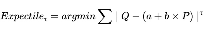
This means we’re adjusting the line so that it best captures the data points at each expectile level.

Now let’s look at our python example. In this example, we are using Kaggle’s retail price csv (link to repo at the end). We will firstly load the data and look at some quantity and price trend per product category.

df=pd.read_csv('retail_price.csv')

##we are interested in price quantity trend based on the same price happend at the same day
agg_df=df.groupby(['product_category_name','month_year','unit_price','holiday','year'],\
                  as_index=False)[['qty','total_price']].sum()

agg_df['if_holiday']=np.where(agg_df.holiday!=0,'1','0')
agg_df['year']=agg_df['year'].astype('str')

fig=px.scatter(agg_df,x='unit_price',y='qty',color='if_holiday',facet_col='product_category_name',facet_col_wrap=2,
           facet_row_spacing=0.1,facet_col_spacing=0.1,opacity=0.6,trendline='lowess',trendline_color_override='blue',
           template='none',title='Product Sales Holiday Analysis',width=600,height=700
).update_traces(
    marker=dict(size=7),hoverlabel=dict(font=dict(size=10))
)

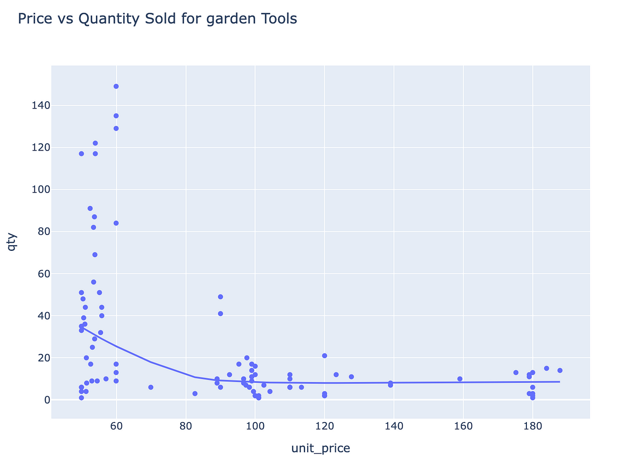
fig.show('iframe')

Our scatterplots show that some products, like Bed & Bath, are price-inelastic (price changes don’t affect quantity). Others, like garden tools, are highly price-sensitive. Let’s explore these patterns more closely using ExpectileGAM to capture different ‘levels’ of demand.

scatterplots of price and quantity for all products

The closer look of price vs quantity for Garden Tools

Next, we fit ExpectileGAM model to each dataset for every product catergory and appened the result together in all_gam_results.

all_gam_results=[]

for p in agg_df['product_category_name'].unique():
    product_data=agg_df.loc[agg_df['product_category_name']==p]
    X=product_data['unit_price']
    y=product_data['qty']
    quantiles=[0.025,0.5,0.975]
    gam_result={}
    for q in quantiles:
        gam=ExpectileGAM(expectile=q)
        gam.fit(X,y)
        gam_result[f'pred_{q}']=gam.predict(X)
    pred_gam=pd.DataFrame(gam_result).set_index(X.index)
    pred_gam_df=pd.concat([agg_df[['product_category_name','unit_price','qty','total_price']],pred_gam],axis=1)
    all_gam_results.append(pred_gam_df)

all_gam_results=pd.concat(all_gam_results)   

Particularly, we look at the prediction result for garden tools product category. The blue line indicates the median prediction at 0.5 expectile level. The gray ribbon defines the upper and lower expectile level at 0.025 and 0.975 expectile levels. The model captures most of the data’s variablities by using three levels of expectile levels, ie. the extreme lows and highs of the data demand.

ExpectileGam prediction visualization for garden tools

We will use the model to predict graden tools specifically and use train_test_split to check the model’s performance.

holiday_encoder = LabelEncoder()
# Fit the label encoders to the categories
agg_df['encoded_holiday'] = holiday_encoder.fit_transform(agg_df['if_holiday'])

# Adding the data
data=agg_df.loc[agg_df['product_category_name']=='garden_tools']
# data['lag_unit_price'] = data['unit_price'].shift(1)
# data['lag_qty'] = data['qty'].shift(1)
# data = data.dropna()  # Drop rows with missing lag values

X = data[['unit_price', 'encoded_holiday']].copy()  # You can add more relevant features
y = data[['qty']].copy()

# split X and y into training and testing sets
X_train, X_test, y_train, y_test = train_test_split(X, y, test_size=0.2, random_state=0)

gams = []
model_train_performance = []
model_test_performance = []
df_gam_results = pd.DataFrame()
quantiles = [0.025, 0.5, 0.975]
for q in quantiles:
    # fit the model on the training data
    gam = ExpectileGAM(expectile=q).fit(X_train, y_train)   
    gams.append({"q": q, "gam_model": gam})
    # predict on the test data
    y_train_pred = gam.predict(X_train)
    y_test_pred = gam.predict(X_test)
    y_pred = gam.predict(X)
    # calculate the performance of the model on the test data
    train_mse = mean_squared_error(y_train, y_train_pred)
    test_mse = mean_squared_error(y_test, y_test_pred)
    # calculate R-squared
    train_r2 = r2_score(y_train, y_train_pred)
    test_r2 = r2_score(y_test, y_test_pred) 
    model_train_performance.append({"q": q, "mse": train_mse, "r2": train_r2})
    model_test_performance.append({"q": q, "mse": test_mse, "r2": test_r2})
    df_gam_results[f"pred_quant_{q}"] = y_pred

We reviewed the model’s performance results and, for the 0.5 expectile level, observed an R² score of 0.54 on the training data and 0.319 on the test data. Not bad for a start! There’s certainly room for improvement through hyperparameter tuning to capture more variance in demand.

model’s train test performance results

Price Optimization

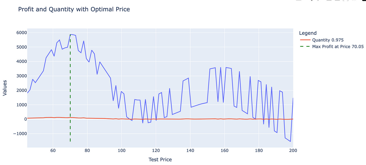
Now, these predictions alone wouldn’t be much help if we couldn’t use them to optimize our prices and maximize profit. For our garden tools subset, the goal is to find the optimal price that brings in the highest profit. Let’s assume our product cost is $20. Using the 0.975 expectile prediction, which gives us a best-case demand scenario, we can estimate the maximum profit possible at different price points.

Maximum profit using 0.975 expectile prediction

Systematic Price Optimization

To systematically find this optimal price:

1. Define a Profit Calculation Function: We calculate profit as (price - cost) * quantity sold using predicted quantities from our GAM model.

2. Set an Objective Function: To maximize profit, we actually minimize the negative profit using SciPy’s minimize() function, setting the bounds to within 20% of the original price to ensure price recommendations are sensible for the business.

3. Iterate Over the Dataset: We then apply this optimization to each price point in the dataset, using the 0.5 expectile level as an example.

Here’s how it looks in code:

# Define a function to calculate profit
def calculate_profit(price, cost, predicted_qty):
    return (price - cost) * predicted_qty

# Add a column for cost (replace this with your actual cost data)
data['cost'] = 20  # For example, assume cost is $5 for all products

# Create an empty column for optimized prices
data['optimized_price'] = np.nan
data['optimized_profit']= np.nan

# Define the objective function to minimize (negative profit)
def objective_function(price, row, gam, cost):
    # Predict the quantity for the current price using the GAM model
    predicted_qty = gam.predict(pd.DataFrame({
        'unit_price': [price], 
        'encoded_holiday': [row['encoded_holiday']]
    }))[0]  # Extract the first value
    
    # Calculate profit for the given price
    profit = calculate_profit(price, cost, predicted_qty)
    
    # We want to maximize profit, so we minimize the negative of the profit
    return -profit

# Create empty columns for optimized prices and optimized profits
data['optimized_price'] = np.nan
data['optimized_profit'] = np.nan

# Iterate over each row in the dataset
for index, row in data.iterrows():
    original_price = row['unit_price']
    cost = row['cost']
    
    # Define the bounds for price (within 20% of the original price)
    bounds = [(original_price * 0.8, original_price * 1.2)]
    
    # Initial guess (start the search at the original price)
    initial_guess = [original_price]
    
    # Use scipy's minimize function to minimize the negative profit
    result = minimize(objective_function, x0=initial_guess, 
                      args=(row, gams[1]['gam_model'], cost), bounds=bounds, method='L-BFGS-B')
    
    # The optimized price is the result
    optimized_price = result.x[0]
    
    # Predict the quantity for the optimized price
    optimized_pred_qty = gams[1]['gam_model'].predict(pd.DataFrame({
        'unit_price': [optimized_price], 
        'encoded_holiday': [row['encoded_holiday']]
    }))[0]
    
    # Calculate the optimized profit
    optimized_profit = calculate_profit(optimized_price, cost, optimized_pred_qty)
    
    # Assign the optimized price and profit to the respective columns
    data.loc[index, 'optimized_price'] = round(optimized_price,2)
    data.loc[index, 'optimized_profit'] = round(optimized_profit,2)

And that’s it! For each original price point, we now have an optimized price and corresponding profit, ready for business decisions.

Optimized_price output

Conclusion

ExpectileGAM is a powerful tool that goes beyond simple averages, helping us understand the full picture of demand. As we’ve seen, it can help optimize prices by factoring in the highs and lows of customer behavior. Try lifting the veils on your data, and see the hidden insights that ExpectileGAM can reveal! Follow me for Part Three, where we’ll dive deeper into optimization, or subscribe to my newsletter to stay tuned!

github source code

---